Using Stars and R to Visualize Curvilinear NetCDF Rasters
Recently, I was working with some netCDF files with raster time-series data in a conic projection. I was doing some calculations with the data and wished to plot the results as a map. The problem was the data file did not include latitude/longitude data for the pixels or a coordinate reference system (crs). The file included metadata which could be used to puzzle out a crs for the xy-indexed grid, but it wasn’t directly readable by any of the R packages I tried, nor did my attempt to build an appropriate proj4 string work out. However, the latitude/longitude coordinates for the pixels were stored in a separate netCDF file but I had a heck of time marrying the data and coordinate files together. This post documents the process I puzzled out and is largely based on this stackoverflow discussion.
Stars is used to read in the netCDF files. Stars and dplyr are used to manipulate the data. Viridis and ggplot2 are used for plotting. Finally, a couple of shapefiles will be pulled from rnaturalearth to provide geographic context to the raster.
library(stars)
library(viridis)
library(dplyr)
library(ggplot2)
library(rnaturalearth)
The data file (“T_LAKE3D.daily.1970.nc”) and the lat/lon file (“Z_LAKE3D.XLONGXLAT.nc”) are read into memory using stars::read_ncdf. Printing the stored objects shows what data is stored in each and what dimensionality it has. Note that stars does not automatically read in all the available variables in a file, so I have specified the relevant variables in this instance.
## Note: Local paths to data read-in elsewhere.
sst <- read_ncdf(path_to_data_file, var = c("T_LAKE3D"))
## Warning in nc_coord_var_finder(dim, var, att, axe, v): missing coordinate
## variables names in coordinates attribute trying to find non-auxiliary coordinate
## variables.## Warning in .get_nc_projection(meta$attribute, rep_var, all_coord_var): No
## projection information found in nc file.## Warning: ignoring unrecognized unit: kcf <- read_ncdf(path_to_coord_file, var = c("XLAT", "XLONG"))## Warning in .get_nc_projection(meta$attribute, rep_var, all_coord_var): No
## projection information found in nc file.sst## stars object with 4 dimensions and 1 attribute
## attribute(s), summary of first 1e+05 cells:
## T_LAKE3D
## Min. :-999.0
## 1st Qu.:-999.0
## Median :-999.0
## Mean :-949.4
## 3rd Qu.:-999.0
## Max. : 277.0
## dimension(s):
## from to offset delta refsys point values
## west_east 1 111 0.5 1 NA NA NULL [x]
## south_north 1 78 0.5 1 NA NA NULL [y]
## soil_levels_or_lake_levels_stag 1 10 0.5 1 NA NA NULL
## Time 1 365 0.5 1 NA NA NULLcf## stars object with 3 dimensions and 2 attributes
## attribute(s):
## XLAT [°] XLONG [°]
## Min. :32.62 Min. :-110.89
## 1st Qu.:38.93 1st Qu.: -95.90
## Median :44.29 Median : -85.00
## Mean :44.30 Mean : -85.00
## 3rd Qu.:49.66 3rd Qu.: -74.10
## Max. :55.70 Max. : -59.11
## dimension(s):
## from to offset delta refsys point values
## west_east 1 111 0.5 1 NA NA NULL [x]
## south_north 1 78 0.5 1 NA NA NULL [y]
## Time 1 1 NA NA NA NA 1The data stored in sst is water temperature data labeled “T_LAKE3D” in degrees kelvin with xy grid index dimensions (“west_east” and “south_north”), lake depth of the temperature estimate (“soil_levels_or_lake_levels_stag”) and time in days (“Time”). So this file contains 365 x 10 raster images–one for each day of the year at each of the ten depth layers.
The object cf stores latitude (“XLAT”) longitude (“XLONG”) in degrees with dimensions for the xy grid and, technically, time (there’s only 1 day in that dimension).
When reading in the data we can also specify how stars should read in the dimensions. For example, we can choose to read in data for a single day at a single depth. Let’s read in the data for January 1st (Time 1) at the lake bottom (depth level 10) using the ncsub option.
sst <- read_ncdf(path_to_data_file, var = c("T_LAKE3D"),
## Specify the layers to read in by dimension. Dimension 3 corresponds to lake
## depth with 10 layers. We'll use layer 10 since its at the lake bottom.
## Dimension 4 is time in days (listed as an index from 1 to 365). We'll grab
## day 1 and read it into memory.
                 ncsub = cbind(start = c(1, 1, 10, 1), count = c(111, 78, 1, 1)))
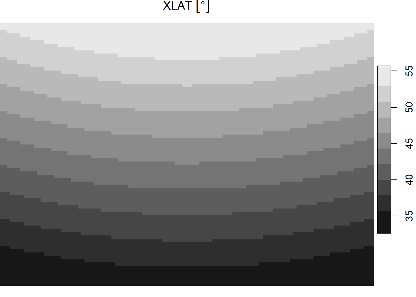
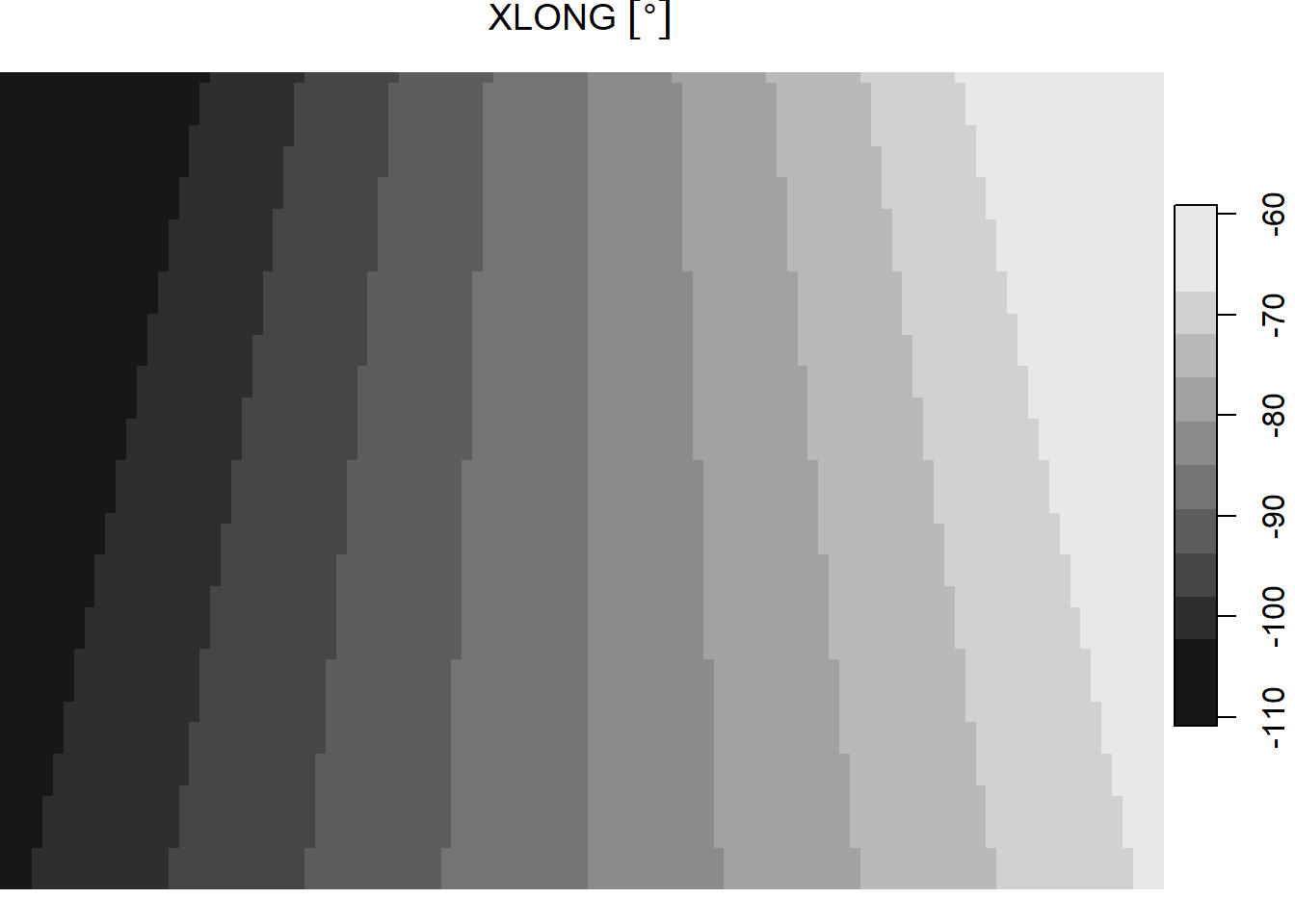
This image is in a conic projection where each pixel has equal area, so the lat/lon coordinates do not form a rectilinear grid–instead they form a curved shape. This can be seen when visualizing the lat and lon values.
plot(cf[1])
plot(cf[2])
Stars has options within the read_* functions for specifying a curvilinear raster. When the lat/lon coordinates are within the data file, one can use the option “curvilinear” to point the function to them. However, in this case, the coordinates are in an external file. The method for overcoming this difficulty is to instead use the function stars::st_as_stars and to point the option “curvilinear” to a pair of matrices storing the lat/lon coordinates. The matrices need to have the same xy dimensionality as the data raster. So, in this case, extract the values “XLAT” and “XLONG” in the object cf and covert them to matrices with the same dimensions as the temperature data. The temperature data grid has 111 columns and 78 rows.
## Convert the lat lon coordinates into matrices with the same dimensions as the
## raster data.
x = matrix(cf[[1]], 111, 78)
y = matrix(cf[[2]], 111, 78)
Next, convert the temperature data with the curvilinear coordinates specified using stars::st_as_stars. We don’t directly use the stars::read_* functions becasue they don’t seem to like be given external curvilinear matrices (or more likely, I was doing something wrong), but st_as_stars handles them just fine.
The curvilinear option needs to be fed a list that assigns the coordinate matrices to the proper dimension variables in the data file–e.g., list(<column_dimension_name> = <latitude_matrix_object>, <row_dimension_name> = <longitude_matrix_object>). Observe that the dimension labels don’t require quotes.
sst <- st_as_stars(sst,
                 curvilinear = list(west_east = y, south_north = x))

sst
## stars object with 4 dimensions and 1 attribute
## attribute(s):
## T_LAKE3D
## Min. :-999
## 1st Qu.:-999
## Median :-999
## Mean :-949
## 3rd Qu.:-999
## Max. : 277
## dimension(s):
## from to offset delta refsys point
## west_east 1 111 NA NA EPSG:4326 NA
## south_north 1 78 NA NA EPSG:4326 NA
## soil_levels_or_lake_levels_stag 1 1 NA NA NA NA
## Time 1 1 NA NA NA NA
## values
## west_east [111x78] -110.89,...,-59.11 [x]
## south_north [111x78] 32.6199,...,55.7044 [y]
## soil_levels_or_lake_levels_stag 10
## Time 1
## curvilinear gridThe data object is now marked as curvilinear and the lat/lon coordinates have been associated with the “west_east” and “south_north” dimensions.
Finally, stars allows one to clean/manipulate data using dplyr operations and magrittr piping. Missing or masked values (e.g., land pixels) are stored as “-999” so we’ll replace those with NA values. I will also convert temperatures from degrees K to degrees C.
sst <- sst %>%
  ## Create a copy of the temperature variable renamed temp, then use select to
  ## drop the original variable as an awkward way to rename the variable.
  mutate(temp = T_LAKE3D) %>%
  select(temp) %>%

  ## Replace the mask values (-999) with NA.
  mutate(temp = ifelse(temp == -999, NA, temp),

  ## Convert temp from degrees K to degrees C.
         temp = temp - 273.15)

sst
## stars object with 4 dimensions and 1 attribute
## attribute(s):
## temp
## Min. :-11.153
## 1st Qu.: -0.440
## Median : 3.379
## Mean : 0.574
## 3rd Qu.: 3.850
## Max. : 3.850
## NA's :8318
## dimension(s):
## from to offset delta refsys point
## west_east 1 111 NA NA EPSG:4326 NA
## south_north 1 78 NA NA EPSG:4326 NA
## soil_levels_or_lake_levels_stag 1 1 NA NA NA NA
## Time 1 1 NA NA NA NA
## values
## west_east [111x78] -110.89,...,-59.11 [x]
## south_north [111x78] 32.6199,...,55.7044 [y]
## soil_levels_or_lake_levels_stag 10
## Time 1
## curvilinear gridThe data summary of temp in the sst object is now much more helpful without the numeric mask values distorting it. It will also plot better without the -999 values.
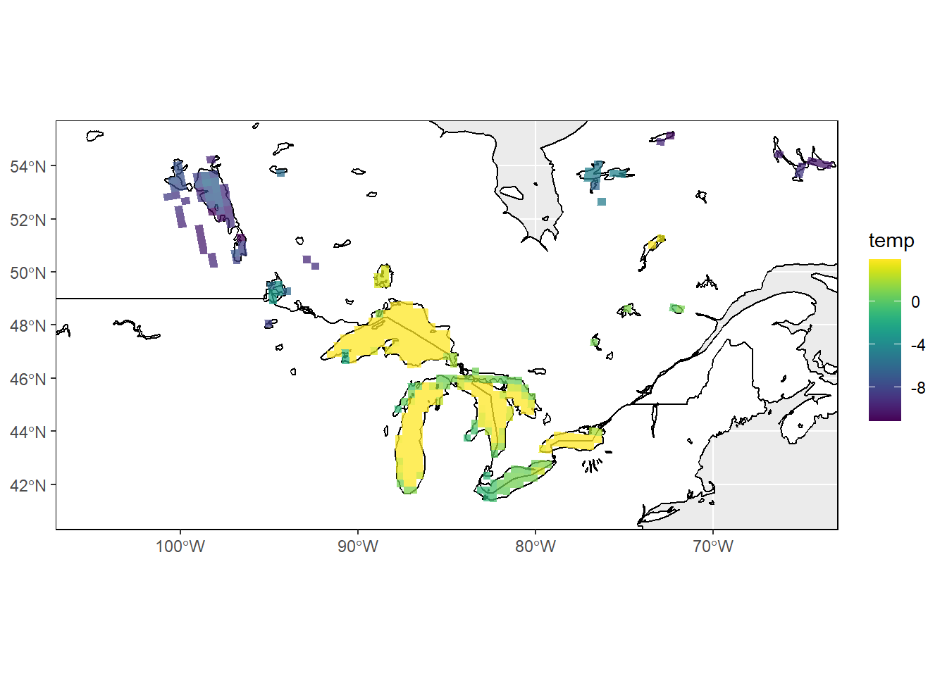
I’ll plot the temp data in ggplot using stars::geom_stars and add in some national boundaries and lake polygons to provide geographic context to the data. I’ll use the viridis package for the temperature color scale.
## Since we have the coordinates, we'll use lat/lon values as crs.
st_crs(sst) <- "+proj=longlat +ellps=WGS84 +no_defs"

## Load contextual map data
world <- rnaturalearth::ne_countries(scale = "medium", returnclass = "sf")
lakes <- rnaturalearth::ne_download(scale = "medium", type = 'lakes', category = 'physical',
                                    returnclass = "sf")
## OGR data source with driver: ESRI Shapefile
## Source: "C:\Users\Lamp\AppData\Local\Temp\Rtmpucrzt8", layer: "ne_50m_lakes"
## with 275 features
## It has 35 fields
## Integer64 fields read as strings: scalerank ne_id## Make sure the crs values are shared by all the mapped objects.
sst <- st_transform(sst, st_crs(world))
## Plot your map
ggplot() +
geom_sf(data = world, color = "black", fill = "white") +
geom_sf(data = lakes, color = "black", fill = NA) +
geom_stars(data = sst, alpha = 0.75) +
coord_sf(ylim = c(41, 55), xlim = c(-105, -65)) +
scale_fill_viridis() +
theme(panel.border = element_rect(colour = "black", fill = NA))
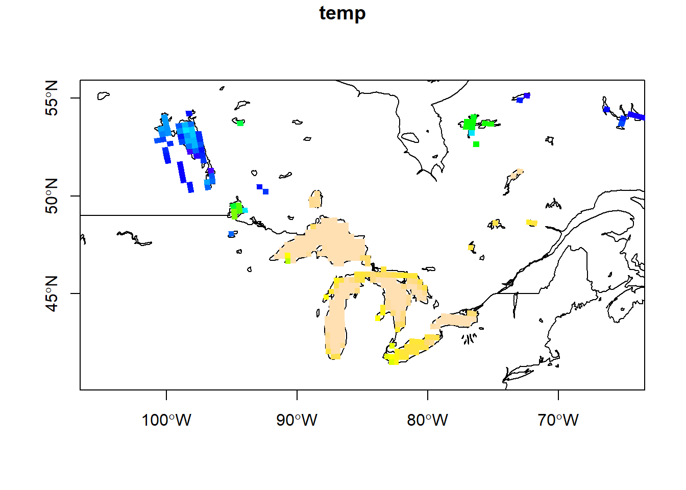
The data can also be visualized with base R plot.
plot(st_geometry(world), axes = TRUE, ylim = c(41, 55), xlim = c(-105, -65))
plot(st_geometry(lakes), add = TRUE)
raster::plot(sst, as_points = FALSE, breaks = "equal", col = topo.colors(100),
     border = NA, key.pos = 1, add = TRUE)